In this tutorial, we’ll show you how to add and format percentage labels to chart in think-cell in three quick and easy steps.
Don’t have the Think-Cell PowerPoint add-on? Read our review to learn more or get a free trial from Think-Cell.com and test it out!
Step 1. Add labels to your chart

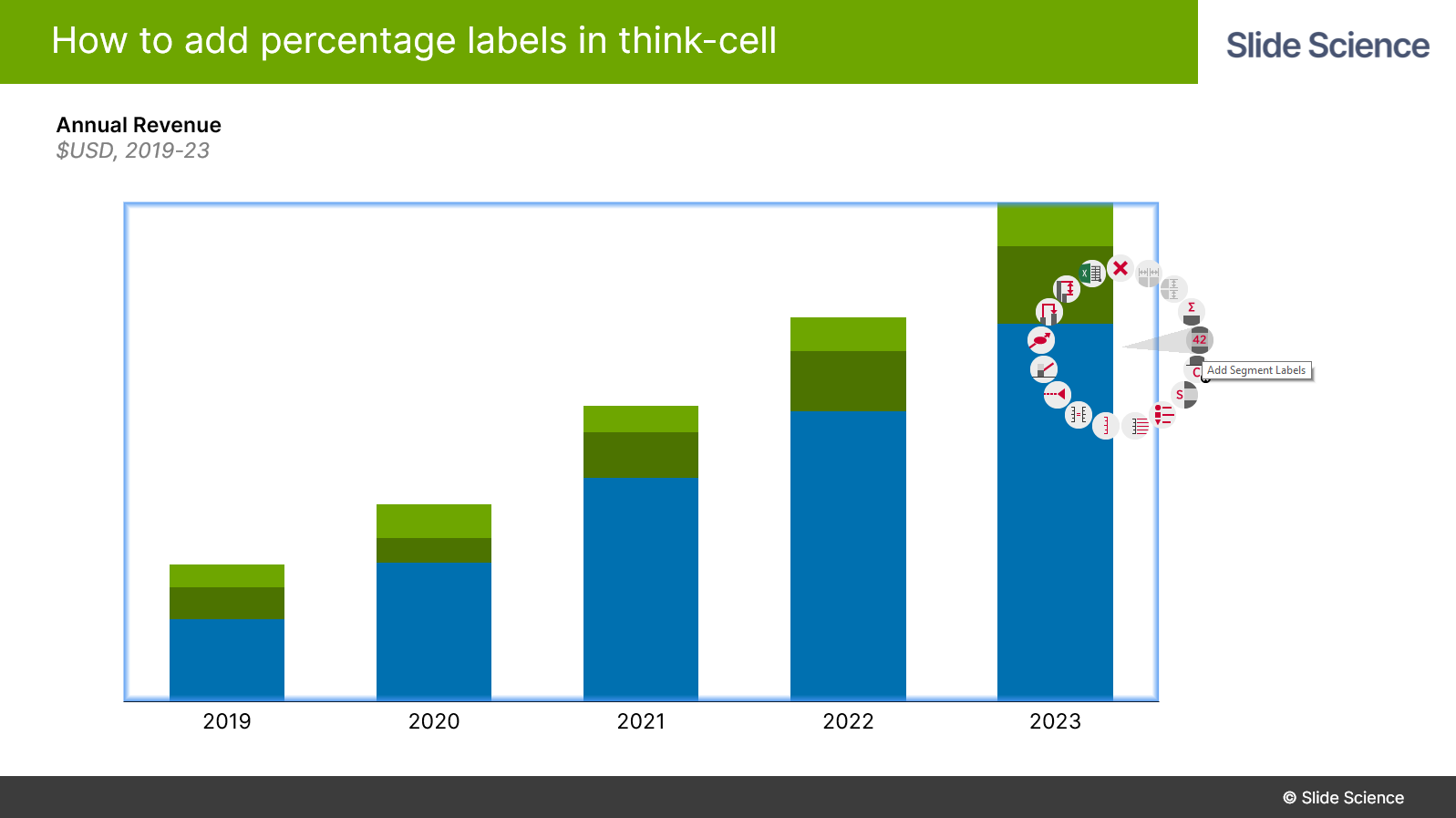
First, you need to add labels to your chart. To add labels to your think-cell chart, right-click on the chart and then select the label type you’d like to add.
In most cases, you will need to add one of the following label types, depending on the chart type that you are using:
- Segment labels: Column and bar charts
- Point labels: Line and area charts
- Inside labels: Pie charts
- Total labels: Column and area charts
By default, your labels will be formatted as integers. In other words, plain numbers with no decimal places.
Step 2. Change the number format to percentage

Next, you need to change the number format of your labels.
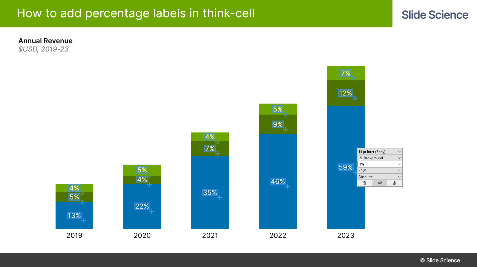
To change your labels to percentage labels, select or multi-select the labels that you want to adjust, and then a formatting toolbar will appear.
In the formatting toolbar, click on the white input box. Then enter an example number in the format that you’d like your labels to have.
It doesn’t matter which specific numbers you use in the input box, it’s only the format that matters. So to add percentage labels, you could write something like 5% or 6.00%. All the labels will be adjusted with the appropriate numbers.
Step 3. Adjust the order of magnitude

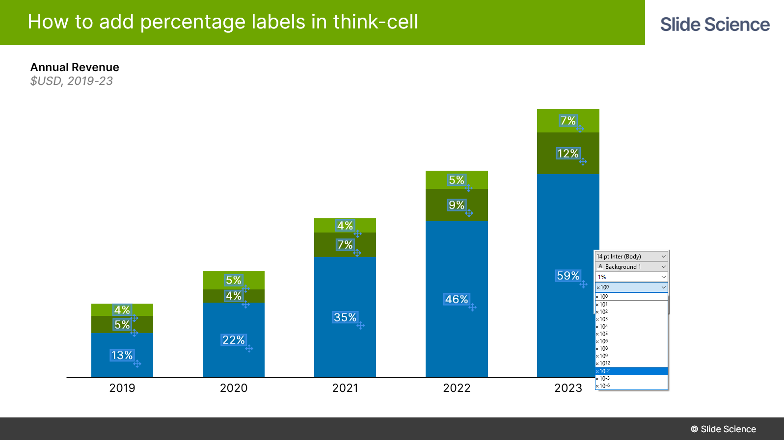
This step only applies in some cases. If your numbers are formatted as decimals in your datasheet, then you’ll also need to adjust the order of magnitude of your labels.
To adjust the order of magnitude of your labels, select your labels again. Then in the formatting toolbar, click on the x100 field, then select x10-2.
